Friday's Quiz Topics

Here’s a list of topics that will be covered on this Friday’s Quiz. I’ll include the relevant homework problems as soon as I get a chance…

Quiz – Sections 4.5-7
Optimization (4.7, #7,11,28)
Calculus and Calculators (4.6, #37)
Analyze a graph based on equation (sketch, etc.) (4.5, #45,59)

I’ll be in early Friday, available after school this afternoon and I’ll check in tonight online. See you in class!

There's no point in being grown up if you can't be childish sometimes.
-Dr. Who

4.7: Optimization Problems!

Hi, everybody. I hope the second day back from cozy break hasn’t been too jarring. Now, it’s that happy time again…time for me to do my blog, and this time it’s on Optimization Problems (which are quite similar to Related Rates, my previous blog).

Optimization are all about maximizing and minimizing something. To untangle all the information given to us in those tedious word problems, we can use a series of steps (Related Rates, anyone?):

1. Read the question carefully. Understand the information you are given and, most importantly, understand what is being asked.

2. Draw a diagram. Label everything. This is not absolutely necessary, but it’s usually helpful.

3. Set up a maximum or minimum equation. This step is kind of like identifying the static equation in related rates. This is the equation that you will modify (Step 5) and differentiate (Step 6).

4. Identify the constraints presented in the problem.

5. Use the constraints to rewrite the equation in terms of a single variable.

6. Find the derivative of the equation. Use this to identify critical points. Remember, critical points are wherever the derivative is equal to zero OR where the derivative is undefined.

7. Test the critical points you found, and the endpoints (these will usually have to do with the constraints), to determine which gives the absolute maximum or minimum.

And, of course, don’t forget to answer the question specifically being asked.

All right, since these are application problems, examples are always extremely helpful.

EXAMPLE 1
Find the point on the parabola y² = 2x that is closest to the point (1,4).

We’re looking for a point (x,y). Since we’re looking for closest distance, we can set up a minimum equation using the distance formula:

d = rad[(x -1)² + (y – 4)²]

This is the distance between the given point (1,4) and the unknown point (x,y).

We are given the equation for the parabola (this is a constraint). We can use this information to solve for x and get rid of the x variables in the equation so we can have an equation in terms of a single variable. (You could also solve for y and substitute that into the minimum equation). Solving for x:

y² = 2x
x = (y²) / 2

We can substitute this value of x into the minimum equation:

d = rad[((1/2)y² – 1)² + (y – 4)²]

To make this equation a little more manageable, we can square it to get rid of the radical:

d² = [(1/2)y² – 1]² + (y – 4)² = f(y)

Now we can differentiate:

f’(y) = 2[(1/2)y² – 1](y) + 2(y – 4)(1) = y³ – 8

Don’t forget about the Chain Rule!!

Now, we have to find our critical points. y³ – 8 is not undefined anywhere. We can look for where it equals 0, though.

y³ – 8 = 0
y³ = 8
y = 2

Now we can use the first derivative test to determine whether y = 2 is an absolute maximum or minimum. You can graph the derivative, or simply think it through. When y is negative, y³ – 8 is less than 2. When y is positive, y³ – 8 is greater than 2. By the first derivative test for absolute extreme values, this means that 2 must be the absolute minimum of f(y).

We have our y value for the point closest to (1,4). To find our x value, we plug in our y value into the equation we solved for x.

x = (2²) / 2 = 2

So (answering the original question): the point on y² = 2x closest to (1,4) is (2,2).

EXAMPLE 2
Find the area of the largest rectangle that can be inscribed in a semicircle of radius r.

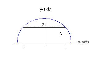
We can draw a picture to make the semicircle the upper half of a circle x² + y² = r² with its center being the origin. The rectangle inside would have a width of y on either side and a length of 2x on either side. Thus, the area is:

A = 2xy

Now we want only one variable. We can solve for y using the equation of a circle:
y² = r² – x²
y = rad(r² – x²)

Substituting this back into our area equation:

A = 2x[rad(r² – x²)] domain: [0, r]

Now we differentiate the area equation:

A’ = 2 rad(r² – x²) – (2x)(1/2)(r² – x²)^(-1/2)(2x)
A’ = 2 rad(r² – x²) – (2x²)(r² – x²)^(-1/2) = 2 rad(r² – x²) – (2x²) / [rad(r² – x²)]
A’ = [2(r² – x²) – 2x²] / [rad(r² – x²)]
A’ = [2(r² – 2x²)] / [rad(r² – x²)]

To find the critical points, we look at where A’ equals 0:
2(r² – 2x²) = 0
2r² – 4x² = 0
4x² = 2r²
x = r / (rad2)

Plug this value of x into the original area equation (remembering that we also solved for y earlier, so we have something to plug in for x and y):

A = 2[r / (rad2)][rad(r² – x²)]
A = 2[r / (rad2)][rad(r² – r²/2)]
A = r²

Before we assume this is our maximum value, we observe the behavior of the endpoints:

A(0) = 2(0)[rad(r² – 0²)]
A(0) = 0
And
A(r) = 2(r)[rad(r² – r²)] = 2r(0) = 0

This confirms that x = r / (rad2) gives us a maximum value of A. Now, to answer the question: the area of the largest inscribed rectangle is r².

The examples we did in class show the optimization problem procedures using more numbers (like the fence area one), whereas these show optimization problems in the coordinate plane, in a slightly more abstract way. It's useful to see this side of the optimization problems, but it's also good to keep in mind that optimization problems can be applied to real world situations. Our homework definitely gives us a chance to work with some, doesn't it?

Here's a link to a website with a lot of sample problems: good practice.

So, if you thought we had icky math tests...take a look at this:
VELOCIRAPTORS!!!!
Ah, yes.

Tessa, you're up next.

Ave atque vale, everyone. ~8)

4-6 Graphing with Calculus and Calculators

Alright, this section is very similar to the previous section in that it deals with the graphs of functions and how calculus allows you to explore those functions. However, this section also talks about the presentation of a graph. Your calculator does not always give you the ideal window, for example. You can use calculus to make sure that you have included all the important parts of your graph in your final window.

Now for a sample problem!
Graph 3x^2-x+2 in a window that includes all important parts of the function.

Our first step is to find out all we can about the function using its first and second derivatives, following the procedure that Jean outlined so neatly in her post.

Increasing on: (0,inf)
Decreasing on: (-inf,0)
Local Maximum: none
Local Minimum: (.167,1.92)
Concave Up: (-inf,inf)
Concave Down: nowhere
Inflection Point(s): (.167,1.92)

You can see that the rather simple graph can be contained in a relatively small window. The ideal window would be something like x=[-2,2] and y=[+0 or -0 or 0,10]. Sorry about that; you got a compliment earlier. Here is the final graph:

Isabella, you are next in line for the joy that is blogging!

For those of you that are wondering, here are the next twenty digits:
pi=...62643383279502884197...

4.5: Summary of Curve Sketching

'Ello, all! God willing, this will be a fairly short post, because, as the title should hint, this section is little more than a "summary" of the previous sections. While 4.1-4.4 laid down the guidelines to drawing and identifying graphs, 4.5 condenses thes guidelines into a nice, easy checklist. Ready for it? Okay:

When sketching a curve...

1. Determine the Domain - It's really helpful to start out knowing where x is and is not defined, so do that first--it'll lay the groundwork for everything else.
2. Determine the x and y intercepts - first, find the y-intercept by plugging in 0 for x. Then, solve for x when f(x) = 0, if the equation isn't too difficult to do so fairly quickly.
3. Determine the symmetry - There are three types of symmetrical functions: even functions, odd functions, and periodic functions. Even functions occur when f(x) = f(-x) and are symmetrical about the y-axis (like cosine graphs and even power functions). If we have an even function, our work is cut in half. We only have to determine the shape of the curve when x is positive. Then we reflect it across the axis and voila! Odd functions, like sine and odd power graphs, occur when f(x) = -f(x) and are symmetrical about the origin. Thus, when dealing with odd functions, we simply determine the shape of the graph when x is positive, then rotate it 180 degrees about the origin. Periodic functions, occur when f(x + p) = f(x) where p is a positive constant called the period. With this graph, we simply have to know what the graph looks like for one interval of length p. Then we can translate that interval to sketch the entire graph. Both sine and cosine graphs are periodic.
4. Find the asymptotes - The three types of asymptotes (only two of which we have seen before) are: horizontal asymptotes, vertical asymptotes, and slant asymptotes. A review of asymptotes can be found in 2.6. Find and draw in the asymptotes.
5. Test for intervals of increase and decrease - To compute intervals of increase and decrese, you need the I/D test, or first derivative test. Find the intervals at which f ' is positive to determine when x is increasing and find the intervals at which f ' is negative to determine when x is decreasing.
6. Calculate local maximums and minimums - By the same first derivative test, you can find the value for which f ' = 0 and note wheter the value is going from negative to positive (minimum) or positive to negative (maximum) or not changing signs (neither local max nor min).
7. Find concavity and points of inflection (POI) - Use the second derivative test to dertermine concavity. When f " is greater than 0, the graph is concave upward, and when f " is less than 0, the graph is concave downward. The point at which f " changes from concave up to concave down (or vice versa) is the POI.
8. SKETCH! - once you've figured out all this information, DRAW away!

Okay, so there's the checklist. Now, let's walk through it with some real numbers. Here's the problem:

Step 1 - Domain/Undefined Values: x is undefined at +/- 1

Step 2 - X/Y Intercepts: the x and y intercepts are both 0

Step 3 - Symmetry: f(-x) = f(x), so the curve is even, which means it is symmetric about the y-axis.

Step 4 - Horizontal and Vertical Asymptotes: this function has both horizontal and vertical asymptotes.

SO, y = 2 is a horizontal asymptote. Now let's look at vertical asymptotes:

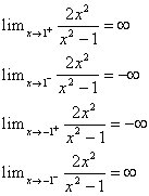
This means that x =1 and x = -1 are vertical asymptotes.

Step 5 - Intervals of Increase and Decrease: Using the first derivative test, we find...

Since f '(x) is greater than 0 when x is less than 0 (and not equal to -1!), and f '(x) is less than 0 when x is greater than 0 (and not equal to 1!), it can be determined that f (x) is increasing between negative infinity and -1, and between -1 and 0, and is increasing between 0 and 1, and 1 and infinity.

Step 6 - Local Maximums and Minimums: f ' (x) changes from positive to negative at 0 and only 0, so that is the only critical number. It is determined, by the first derivative test, that it is also the local maximum.

Step 7 - Concavity and Points of Inflection:

Thus, the curve is concave upward between negative infinity and -1 and between 1 and infinity, and concave downward between -1 and 1. Because 1 and -1 are not in f's domain, it has no points of inflection.

Step 8 - SKETCH!: now, take all of the bolded conclusions drawn from the previous 7 steps and sketch a graph that works with those conclusions. Got it? Good!

For more practice or a second opinion, a this is a great site.

Yay for short blogs! Actually, it got rather long, didn't it? Long but all summary, a nice simple section. Have a nice weekend, you guys!

I can't help but wonder... was this what Mr. French was like when he was little?

Your turn, MARK!

Friday's Quiz Topics

Here’s a list of topics that will be covered on this Friday’s Quiz. I’ll include the relevant homework problems as soon as I get a chance…

Quiz – Sections 4.1-4
Find critical numbers of a function (Sec. 4.1, #41)
Verify a function satisfies conditions of Rolle’s Theorem or the Mean Value Theorem, then solve for “c” (Sec. 4.2, #1,11)
L’Hopital’s Rule – evaluate limits (Sec. 4.4, #15,21,47)
Sketch a graph given continuity and max/min conditions (Sec. 4.1, #7,11)
Analyze a function given an equation: determine increasing/decreasing intervals, max/min values, concavity intervals, points of inflection (Sec. 4.1, #29,49, and any of the questions in Sec. 4.5)
Analyze and draw a graph of a function given the graph of the derivative. (Sec. 4.3, #5,7,31)

I’ll be in early Friday. See you in class!

"Seven days without laughter make one weak."
-Joel Goodman

4.4 Indeterminate Forms and L'Hospital's Rule

Hey everyone. I guess I’m here to help you all learn about the wonders of section 4.4 – Indeterminate Forms and L’Hospital’s Rule.

The point of this lesson is to find out what’s going on near the ends of the graph at infinity.

Okay, I guess we’ll be doing an example problem to learn this lesson quickly.

Example Problem:

We’re going to solve this using L’Hospital’s Rule:

***L’Hospital’s Rule***

Suppose f and g are differentiable and

g’(x)≠ 0 near a (except possibly at a). Suppose that:

and

or that

and

(In other words, we have an indeterminate form of typeor

or

If the limit on the right side exists (or is infinite or negative infinite).

Now, you always have to remember that the limit at infinity depends on how fast the top grows compared to how fast the bottom grows. And another thing to keep in mind, L’Hospital’s Rule can only be used when the limits are indeterminate.

There are 7 indeterminate forms of limits that we know of:

or

or

Although there are 7 indeterminate forms of limits, it’s usually best to try to change any the last 5 forms to one of the first two forms :

Now…you may be asking, “HOW do we do this?” It’s simple. First of all, we can see that if we had left the equation (ln x) / (x-1) alone and tried to find the limit by simply plugging “infinity” into ‘x’, the limit would become infinitely large. Eventually, “ln x” would become “infinity,” and “x-1” would also become “infinity.” Hopefully you realize that is one of our indeterminate forms. Now we know that we can use L’Hospital’s Rule!

So using L’Hospital’s Rule, we rewrite the derivative of “ln x” as (1/x)(1) and the derivative of “x-1” as 1.

To find the derivative of this whole limit of a function, we don’t use the quotient rule. Instead, we take the derivative of the top (ln x) and divide it by the derivative of the bottom (x-1).

Eventually, we can find that the limit, as x approaches infinity, is zero.

To simplify the definition of L’Hospital’s Rule, here’s an equation to help you figure this thing out:

Well, I hope you understand all of this…but in case you don’t, we’ll try some different problems that use The Rule (sorry, I just don’t want to constantly type out L’Hospital’s Rule…which I just did…again. AHHHHHH!!!).

Example:

Using THE Rule, we find that the derivative of (3x² + 4) is 6x, and the derivative of (2x² + 7) is 4x. So we just put the top derivative over the bottom derivative, like this , cancel out the x’s, do some simplifying…and PRESTO! We find that the limit is: Another problem like this:

We used the Rule to find that the limit, as x approaches infinity, is 4! Huzzah!

Okay, last sample problem…this one’s a little different from the last two we’ve had.

Example:

Without using the Rule, we would find that the limit would be:

Now, don’t make this mistake. Although you might think that zero multiplied with negative infinity would equal zero, it doesn’t. Zero multiplied with negative infinity is actually an indeterminate form of limits. That means that we can use the RULE!

So we will re-do this whole thing using L’Hospital’s Rule:

First, let’s start off by showing that the limit becomes an indeterminate form of limits.

We can rewrite x so that it does not end up equaling zero.

X =

Now that this is in an indeterminate form that we like, we use L’Hospital’s Rule:

Derivative of (ln x) divided by the derivative of (x^-1) So we see that as x approaches 0 from the right side, the limit becomes -(0).

And no, Jean, this does not “become negative zero”…it is simply zero.

Hopefully you all understand this lesson now because I know I DO!

BUT, in case you still need help, you can go to these sites:

Site#1

or

Site#2

Even though I had such a fun time using Equation Editor 41 times and uploading 35 pictures multiple times, it is definitely time to stop before I get addicted to blogging. So here’s a reminder to Jean that she is up next! Hurrah!


sorry about the blacked out equation...you can just click on it to see the equation...o, and sorry about this blue-underlined sentence...I don't know why it's doing this, but it's really annoying and I want it to stop...but it won't. So....I can't do anything.

4.3: How Derivatives Affect the Shape of a Graph

The title for Section 4.3 is, in my opinion, quite vague. The concepts, however, are specific, and they clear up a lot of things, such as what derivatives and second derivatives actually mean with respect to a graph's appearance. Let's get started. We'll talk first about, well, first derivatives.

The Increasing/Decreasing Test is another one of those things that's quite simple and easy once you hear it, like the Intermediate Value Theorem. It states that

1) If f ' > 0, then f is increasing, and
2) If f ' <>

This makes perfect sense, because we know that f ' represents the slope of the line tangent to f. So, if the slope of f is positive, the y-values must be increasing as the x values increase, and if the slope is negative, the y-values must be decreasing as the x-values increase.

Now, we have the First Derivative Test, which is pretty self-explanatory. For this test, we must first have c represent a critical point on the function f. Reminder: a critical point is a point on the graph of f where either f '(c) = 0, or f '(c) does not exist.

The First Derivative Test says ...
1) If f ' changes from positive to negative at c, then a local maximum of f is at c.
2) If f ' changes from negative to positive at c, then a local minimum of f is at c.
3) If f ' doesn't change signs at c, then there is no local maximum nor local minimum of f at c.

All right then, let's move on to second derivatives. We know that while the first derivative tells us where a function increases and decreases, the second derivative (the derivative of the first derivative) tells us how the slope of the original function changes.

Before talking about how the second derivative affects a function, we must first define concavity, because, as I’ll explain momentarily, it relates to second derivatives.

On an interval, the graph of f is concave up when its tangents lines lie below the curve,
And the graph of f is concave down when its tangent lines lie above the curve.

That being said, we can use the second derivative to determine where a graph is concave up or concave down. The Concavity Test says …

1) If f ">0, then the graph is concave up.
2) If f "<0,>

As a side note, a point of inflection, a concept we learned in Precalc whose origins were somewhat fuzzy, is a point on a graph f at which the curve changes concavity, or, in other words, where f " changes signs.

The Concavity test leads us to our Second Derivative Test, which states ...

At a critical point c, with f '(c) = 0,
If f "> 0, then a local minimum of f is at c, and
If f "<>f is at c.

Mr. French gives us a helpful and, I must admit, quite fantastic way to remember this. If f "> 0, or, in other words, if f" is positive, then it is happy, and makes a Smiley Face. The Mouth of a Smiley Face is concave up, and therefore has a local minimum. Huzzah for pneumonic devices!

EXAMPLE

With the information I just explained, we can easily sketch the graph of a function.
Let's try y = (x^5) - 5(x^4)

First, find the first a second derivatives.

y' = 5(x^4) - 20(x^3)
y" = 20(x^3) - 60(x^2)

Next, factor the first derivative and find the zeros to find the graph's critical points. Don't forget to check for place where f ' does not exist. We know there aren't any critical points like that with this function, because it is a polynomial.

y' = 5(x^4) - 20(x^3) = 5(x^3)(x - 4) ==>The critical points are at x=0,4.

Next use either the first or second derivative test to determine whether they are maximums or minumums. Personally, I advocate the second derivative test, as it is much faster and simpler. Plug in the x values to the equation for the second derivative.

y" = 20(x^3) - 60(x^2) = (20(0)^3) - (60(0)^2) = 0. This is neither positive nor negative, so there is neither a maximum nor a minimum.
y" = 20(x^3) - 60(x^2) = (20(4)^3) - (60(4)^2) = 320. This value is positive, so there is a local minimum.

Now, let's plug 0 and 4 into our original equation to find the coordinates. When we do this, we get the coordinates (0,0) and (4, -256).

Next, factor the equation for the second derivative to find the critical points. In the second derivative, the critical points are places where the original function may change concavity, having a point of inflection.

y" = 20(x^3) - 60(x^2) = 20(x^2)(x - 3) ==> The critical points are at x= 0,3. By plugging in values between and outside of those points, we find that before zero, the second derivative is negative, between zero and three, it is still negative, and beyond three, it is positive. Thus, the graph of y changes from concave down to concave up at x=3. By plugging into the original equation, we find that the specific point of inflection is (3,-162).

Now that we know our points of inflection, the specific local minimum, where the graph is decreasing and increasing, and where it is concave up and concave down, we may sketch the function. Using these new processes, we can break down complicated functions to their essential pieces of behavioral information, and use those essential pieces to sketch.

Here is a website that explains quite well how second derivatives relate to concavity and points of inflection.

John the Prophet, you are now John the Scribe for Lesson 4.4 tomorrow. Don't forget!

Here's some advice that I think we could all do good to hear every once in a while. It comes from the hilarious Douglas Adams.

Chapter 3 Test, #10

Sorry I'm late, guys.

Anyway, the problem gives us the function



and asks us to find



In order to do this, let's first find the higher order derivatives of the function. Remember the chain rule!

The derivative of cos(2x) is:



Find the next derivative:



And the next:



Finally, it repeats itself, but with a higher coefficient.



So, since it repeats at the fourth derivative, we divide the derivative we are looking for, 1428, by 4. And, conveniently, 4 goes into 1428 evenly. This means that we have to use the 4th derivative equation. If you will notice, with each derivative, the coefficent is two to the the power of the number of the derivative.

So, the equation is



And there you have it!

Formal Complaint

I'd like to file a Formal Complaint, Mr. French. Why is it that the AB Calculus C Blog gets to have BACKGROUND MUSIC and ours doesn't? WHAT TYRANNICAL INJUSTICE.

Chapter 3 Test, problem 13

At noon, ship A is 200 km west of ship B. Ship A is sailing south at 34 km/hr and ship B is sailing north at 21 km/hr. How fast is the distance between the ships changing at 8:00 pm? Round the result to the nearest thousandth if necessary.

Step 1: Draw a picture and label all the parts.
The picture will be inserted on Tuesday...oh the mac fun.

Step 2: Find the static equation. Then plug in all constants.
(x^2) + (y^2) = (d^2)
(200^2) +(y^2) = (d^2)

Step 3: Find the information provided.
x = 200 km = constant
t = 8 hrs
y = (21 km/hr)(8 hrs) + (34 km/hr)(8 hrs) = 440 km
(d^2) = (200^2) + (440^2)
d = 483.3218 km
dy/dt = 34 km/hr - (-21 km/hr) = 55 km/hr

Step 4: Find the dynamic equation. Then plug in all known information.
0 + 2y(dy/dt) = 2d(dy/dt)
2(440 km)(55 km/hr) = 2(483.3218 km)(dd/dt)
dd/dt = 50.070 km/hr

Answer = 50.070 km/hr

SEE YOU ALL AT PREPSTOCK I HOPE!!!

Chapter 3 Test # 2

Differentiate:
y = e^cos(3x)

Solution: Remember to use the CHAIN RULE!
1) Differentiate the outside function.
e^cos3x
2) Multiple solution from #1 by the derivative of the inside function.
(e^cos3x)(-sin3x)
3) We must also use Chain Rule for -sin3x. So....
(e^cos3x)(-sin3x)(3)
4) So...
y' = -3(e^(cos3x)) * sin(3x)

Answer to Chapter 3 Test, #8

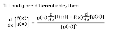
This is a quintessential Quotient Rule problem. We all remember Quotient Rule?

So first let’s find all of the pieces we need:

Numerator (“HI”): u
Denominator (“LO”): u2-1
Derivative of Numerator (“dHI”): 1
Derivative of Denominator (“dLO”): 2u

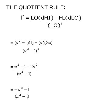
Now it's just simple plug-and-chug.



Yahoo!

Chapter 3 test, Question # 12

a) Use linear approximation techniques to estimate 256.8^(1/4). Leave your answer as a number plus or minus a fraction. Show your work.

b) Determine the calculator-generated value of 256.8^(1/4).

c) To how many decimal places is your estimate similar to the calculator-generated value?

Solutions
First make a general equation: f(x) = x^(1/4)
Find the derivative of that function: f’(x) = (1/4)x^(-3/4)
Choose an a close to the original x-value that gives a nice answer: a = 256
Substitute the a-value into f(x): f(a) = 4
Substitute the a-value into f’(x): f’(a) = (1/4)256^(-3/4) = 1/256
Use the equation for linear approximation: L(x) = f(a) + f’(a) (x-a)
L(x) = 4 + (1/256)(.8) = 4 + (1/320)


a) Answer: 4 + (1/320)

Enter in calculator: 256.8^(1/4) = 4.00312…
b) Answer: 4.00312…

Compare the two answers
c) Answer: 5 decimals

Test Question #7

Test Question #7

U(x) = (8x + 4)^11 (7x2 + 9x – 4)^3

This problem requires both the product rule and the chain rule.

U’(x) = ((8x + 4)^11) (3(7x2 + 9x – 4)^2 (14x + 9) + ((7x2 + 9x – 4)^2) (11(8x + 4)^10) (8)

So, In words…

It is the first half (8x + 4)^11

Times the derivative of the 2nd half (7x2 + 9x – 4)^3 [Remember chain rule!!]

Added to

The 2nd half (7x2 + 9x – 4)^3

Times the derivative of the fist half


ALL SET!!!

O, by the way, all of these equations looked absolutely brillant on my incredible MAC, but seeing as blogger is biased against MACs, and gives undeserved preferential treatment to PCs, my equation now looks like I am a 5th grade computer skills failure. Just thought you might want to know.

-Lauren

Chapter 3 Test, Question # 5

5) Find the derivative of the following function: y = 9^7x


Ok so first we should realize that there is a variable in the exponent. So, we need to bring the x variable down by using logarithmic properties.

Step #1: Take the ln (natural log) of both sides of the equation. The property states: lnb(x^n) = n lnbx. Then we have the equation: ln y = (7x)(ln9).

Step #2: Take the derivative of new equation. The derivate is: (1/y)(y') = (7)(ln9)

Step #3: Isolate or solve for the y' by multiplying both sides by y. Then we get: y' = 7(ln 9)(y')

Step #4: We're almost there! Now dont forget to replace the y with the original function. The final answer is y' = (7)(9^7x)(ln9). The answer was B!!!

Be careful in this problem! DONT USE THE POWER RULE! Choice number A was the answer if we had taken the power rule...which is wrong wrong wrong!

Hope that helped everyone! Good luck.

Test Question #17

#16
So, once you have completed #14, you have the two equations v=-4t^3+12t^2 and a= -12^2+24t. You graph those two equations and find all the zeroes because these points are the points at which the particle is changing from speeding up or slowing down to slowing down or speeding up.


When the particle is slowing down, the velocity will be positive and the acceleration will be negative, or the velocity will be negative when the acceleration is positive. For t<0, velocity is positive and acceleration is negative, so this is part of our final domain. At t=2, acceleration becomes negative while velocity is still positive. But at t=3, velocity becomes negative. So, this can be written 2<t<3. The correct notation for the final domain is t<0 U 2<t<3.

Chapter 3 Test, Question #1

Differentiate:


Here we must first recognize that we are dealing with the product rule, meaning that we must multiply the derivative of the outside function by the inside function and then add the outside function times the derivative of the inside function. So:

Derivative of is by the derivative of exponential rule.

Derivative of is by the definitions of trigonometric derivatives.

Therefore by putting the information we have into the product rule, we get:



which, rearranged, looks just like answer (c) which is: